An Extended SIR model with Vaccine Dynamics for SARS-CoV-2 adaptation rate
R.Horvat*, T.Surić *
Division of Experimental Physics ,Ruđer Bošković Institute, Bijenička 54, 10000 Zagreb, Croatia.
*Corresponding author
*R.Horvat ,Division of Experimental Physics ,Ruđer Bošković Institute, Bijenička 54, 10000 Zagreb, Croatia.
E-mail:horvat@irb.hr
DOI: 10.55920/JCRMHS.2022.02.001060

where m is the viral mutation rate per capita per unit time, I(t) is the proportion of infected/infectious people in the population at a time t, R(t) is the proportion of the population who had recovered from a disease and acquired immunity at a time t and V(t) is the proportion of the population who had been vaccinated and acquired immunity at a time t. Here the sum, where N is the total number of people in the population, represents a net immune response of the population at a time t. The potential for transmission of these mutations (termed as Evolutionary Infectivity Profile (EIP) in [4]) to the susceptible compartment S(t) must be proportional to I(t), hence

Note that EIP(t) weighs the average amount of viral adaptation transmitted to the susceptible compartment at a time t after the onset of the infection. Further, if the number of the infected tends to zero for large times, the EIP would do the same. We shall show in the following that for an infectious disease with a short duration immunity and for a low vaccination rate, this might not be the case. This would inevitably get us into a potentially dangerous situation, in which a virus changes quickly. Trevor Bedford was the first to think, admittedly heuristically, about this problem for the SARS-CoV-2 virus [5].

where is the rate of recovery from infection and R0 is the basic reproduction number. The initial conditions at the onset of the infection are , and , where the parameter represents the reduction in transmission due to the presence of the fraction of the vaccinated in the population at the onset of the infection. The effective reproduction number Reff = (1-f) R0 is established at t=0 in our simplistic model. Note that as the stock of vaccinated people stays constant over time, it does not enter the equations, but should be present kinematically in order to express the constancy of population N at any moment. Formally, for later use in a more general discussion, we may introduce the compartment of the vaccinated V(t) and set , with . For , S, I and R approach their asymptotic values , and , where and are determined from the condition , which is a simple transcendental equation for .
In Fig. 1 we have drawn a plot with the viral abundance I(t) on the y-axis, and the population immune pressure, , on the x-axis. We shall call it the Viral Abundance - Immune Pressure (VA-IP) diagram. The hyperbolas on the plot are the curves on which the product stays constant, rising from the bottom up. Note that when we switch from f = 0 to a finite f, the viral adaptation rate penetrates less and less into the curves with ever increasing values, as we increase f. Also the EIP switches off for large times for any f, as the compartment I(t) eventually empties off. As f is increasing, the maximum of shifts towards larger times, but the number of accumulated mutations always decreases. However the EIP shows an interesting feature (see Fig. 2). We see that curves with various f”s do cross each other at some instant of time. This is due to the fact that the more vaccinated people there are in the population, the later the maximum of infection will be attained. The potential for transmission of virus mutations at late time is thus larger in the vaccinated case. In our figures we have taken , a lower limit for the highly contagious and predominant SARS COV2 variant nowadays, the Omicron. We have also taken for the infectious period to be 4 days.

Figure 1: The epidemic dynamics described by the SIR model, Eq. (3), is illustrated in the VA-IP diagram with I(t) on the y-axis, and the population immune pressure, , on the x-axis. The lines show the epidemic dynamics for f=0 (full line), f=0.3 (dashed line) and f=0.5 (dot-dashed line), , γ=1/4 . In these cases the epidemic starts with , and ends with. The dotted hyperbolas represent lines with the constant adaptation rate .

Figure 2: EIP, Eq. (2), calculated within the SIR model as a function of time for f=0 (boxes), f=0.3 (diamonds) and f=0.5 (triangles), , γ=1/4 . Initial conditions are the same as in Fig. 1.
AN EXTENDED MODEL WITH VACCINE DYNAMICS AND SHORT DURATION IMMUNITY
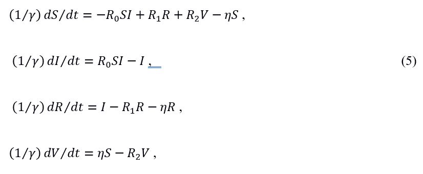
We define our model with vaccine dynamics and short duration immunity by the following set of differential equations:

where , , , is the rate of losing immunity vested by getting over a disease, is the rate of losing immunity vested by vaccination (the rate at which those people are being vaccinated is modulated by vaccine efficacy for transmission ) and is the rate at which susceptible and recovered people acquire immunity by vaccination . The parameters and R0 are the same as in Eq. (3). The stock of vaccinated people splits as . The same is assumed for both and.
An important remark is in order at this point. There is a reason we have had to split the compartment of vaccinated individuals into the two, and , both of which obey a separate differential equation. We could have joined the last two equations into a single one (modifying the rest of the equations accordingly),

but in this case the model would be accurate only if . In (5), after a time had elapsed, the compartment of the vaccinated emptied out entirely into the compartment of the susceptibles. This is altogether consistent if . But for our set of equations should provide for a possibility for the compartment of the vaccinated to empty out into the compartment of the recovered as well, since the duration of naturally vested immunity lasts longer than the duration of immunity vested by vaccination. Otherwise an individual with (for instance) a lifelong immunity () would be driven, through vaccination, again to the susceptibles, supporting thereby an endless cycle of infection. This obviously does not make sense. So in what follows we will stick to the set (4), as it works for any and .
As in the previous case, Eq. (3), as , S, I , R , VS and VR will approach their asymptotic values S(∞), I (∞), R(∞), VS (∞) and VR(∞). In general I (∞) can be different from zero. These asymptotic values are obtained (except for some special cases when either or is zero) as the solutions of some simple algebraic equations. Two general cases are distinguished, depending on which may have a critical value

These stationary solutions can be endemic () or disease-free (). For the asymptotic values read:

The effective reproduction number asymptotically equals 1 () or less than 1 ().

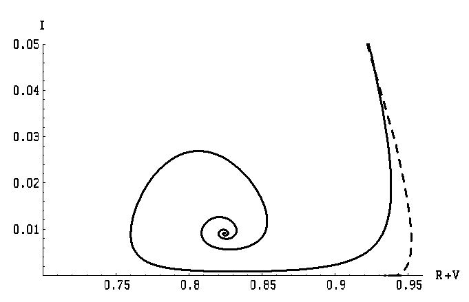
Figure 3: VA-IP diagram for the extended model, Eq. (4). The lines show the epidemic dynamics for two different ζ rates: a subcritical ζ=0.004 d-1 (full line) and a supercritical ζ=0.04 d-1 (dashed line). In these cases the epidemic starts with , , γ=1/4 d-1 , γ1= γ2=1/180 d-1 . The critical rate, where is given by Eq. (6). The dotted hyperbolas are the same as in Fig.1.

Figure 4: Blown-up version of the Fig. 3 in the vicinity of the curves’ endpoints.

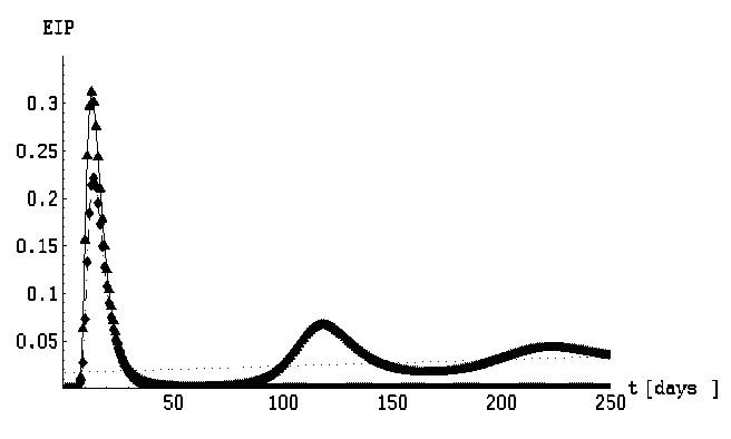
Figure 5: EIP(t) function in the extended model, Eq. (4), the parameter space being the same as in Fig.(3) . The subcritical EIP(t) (ζ=0.004,triangles) behaves as a straight line (dotted line) with a positive gradient in the limit. The supercritical EIP(t) (ζ=0.04, diamonds) vanishes as .
It is clearly seen from Eq. (2) that EIP behaves as a straight line in the limit, and we take its gradient to be a measure of how much of viral adaptation is being transferred to S(t), when stationary states are reached. In Fig. 5 we have depicted the EIP for two values of , one subcritical and the other supercritical. In the supercritical case the gradient is zero, meaning not only that a disease is under control but also that viral adaptation stops being transferred soon after the maximum of infection is attained. Conversely, in the subcritical case the gradient is different from zero, signaling not only that a disease is not under control, but also that viral adaptation is being transferred to a susceptible population all the time. In the latter case the number of advantageous mutations grows with time. In Fig. 6 we have shown again the subcritical case retaining the same parameters as in Fig. 5, but now any vaccination is excluded, i. e. = 0 is set. We see a noticeable increase of the gradient in this case, showing that even the low rate vaccination helps in the non-proliferation of viral adaptation through a population.

Figure 6: EIP(t) with no vaccination (ζ=0), and other parameters being the same as in Fig. 5. EIP (t) approaches a straight line as.
In Fig. 7 we have shown the EIP for two different values of, but now with both values being supercritical. We see a somewhat different pattern of that in Fig. 3 when we increase (analog to increasing f there). Apparently the curves do not cross each other, and the potential for transmission of viral mutations shows no tendency to grow at late time for larger. We have also explored large portions of the parameter space from the both sides of = and found no qualitatively different outcomes.

Figure 6: EIP (t) for two supercritical cases: ζ=0.03 (diamonds) and ζ=0.08 (triangles), and the other parameters being the same as in Fig. 5. EIPs vanish as.
Finally, a note about vaccine efficacy (for transmission) in our examples is in order. In our examples we have taken both types of immunity to last for six months, pinpointing the critical rate to be 0.0278. This means that almost 3% of the population should acquire vaccine-induced immunity each day. Since the present day vaccines have a pretty low efficacy for the Omicron variant, this means that much more than 3% of the population should be vaccinated each day in order to maintain a disease-free status and prevent further viral mutations. At present this is difficult to achieve for most countries, especially the poorer ones.
Statements and Declarations
Funding: None
Conflict of interest: None declared
- Andreas Handel, Ira M. Longini Jr, Rustom Antia: What is the best control strategy for multiple infectious disease outbreaks? Proc. R. Soc. B (2007) 274, 833-837; doi:10.1098/rspb.2006.0015
- Anderson RM, Vegvari C, Truscott J, Collyer BS: Challenges in creating herd immu-
nity to SARS-CoV-2 infection by mass vaccination, Lancet 2020; published online Nov 4. http://dx.doi.org/10.1016/S0140-6736(20)32318-7. - Zhu, N., Zhang, D., Wang, W., Li, X., Yang, B., Song, J., Zhao, X., Huang, B., Shi, W., Lu, R., et al. (2020): A novel coronavirus from patients with pneumonia in China, 2019, New England Journal of Medicine 382, 727-733.).
- Bryan T. Grenfell, Oliver G. Pybus, Julia R. GogJames, L. N. WoodJanet, M. DalyJenny, A. Mumfordand, Edward C. Holmes, Science, 16 Jan 2004, Vol 303, Issue 5656, pp. 327-332; DOI: 10.1126/science.1090727
- Twitter posts 1-19 on Nov 22, 2021
- Anderson, R. M.; May, R. M. 1991,Infectious diseases of humans dynamics and control, Oxford, UK: Oxford Science Publications
- Hethcote, H.W. 2000,The mathematics of infectious diseases, SIAM Rev. 42, 599-653. doi:10.1137/S0036144500371907
